

Bronze, silver, gold is usually drawn as three boxes and an arrow. The boxes are not the point; the promises are. Bronze promises that nothing was lost. Silver promises that every row still present passed a written rule, and every row that failed one can be found. Gold promises that the table answers one question, in the shape the question is asked. This is what those promises look like on a dataset that is public, free and dirty in exactly the ways production data is dirty: the NYC Taxi and Limousine Commission trip records, on Databricks.
The dataset
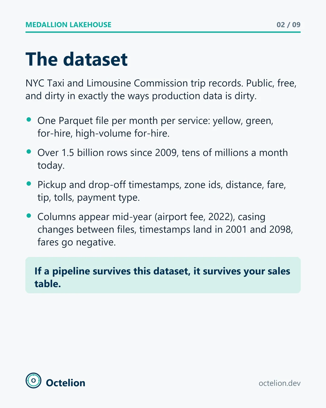
The TLC publishes one Parquet file per month per service: yellow, green, for-hire and high-volume for-hire. That is more than 1.5 billion rows since 2009, and tens of millions a month today across the four services (the yellow file alone is about 4.3 million). Each row carries pickup and drop-off timestamps, zone ids, distance, fare, tip, tolls and payment type.
It also carries every problem a pipeline has to survive. Columns appear mid-year (the airport fee arrived in 2022). Column casing changes between files. Timestamps land in 2001 and 2098. Fares go negative. There is no trip id. If a pipeline survives this dataset, it survives your sales table.
Bronze: land everything, drop nothing
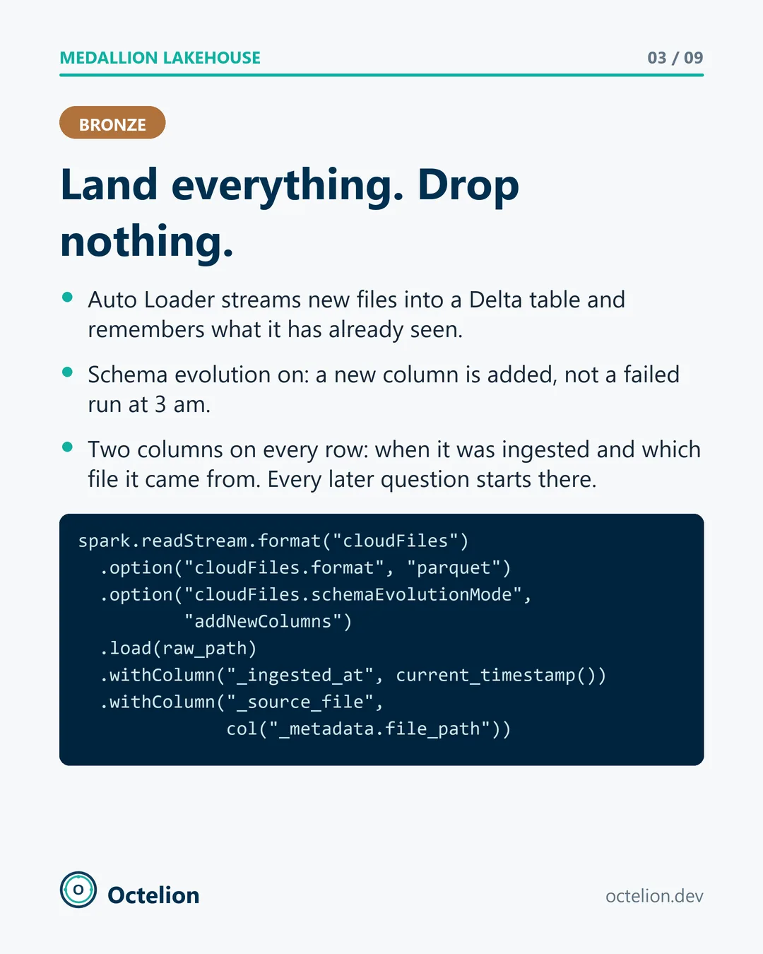
The first layer has one job: get every file in, exactly as it arrived, and remember that it did. Auto Loader streams new files into a Delta table and remembers what it has already seen, and with allowOverwrites on a republished month is picked up again without a manual step. Schema evolution is on: a new column is added to the table, not reported as a failed run at 3 am. This is the whole of the bronze code on the slide:
spark.readStream.format("cloudFiles")
  .option("cloudFiles.format", "parquet")
  .option("cloudFiles.schemaEvolutionMode", "addNewColumns")
  .load(raw_path)
  .withColumn("_ingested_at", current_timestamp())
  .withColumn("_source_file", col("_metadata.file_path"))
Two columns go onto every row at this point: when it was ingested and which file it came from. Every later question about a strange number starts there, so they are added before anything else touches the data. Nothing is filtered in bronze. The negative fares and the trips from 2098 go in. Bronze is the evidence, and you do not edit evidence.
Silver: fix what can be fixed, quarantine the rest
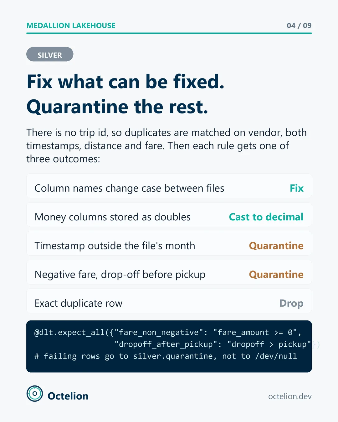
Silver is where rules live, and each rule gets one of three outcomes. Some problems are fixed: column names are normalised, money columns are cast from double to decimal. Some rows are dropped: exact duplicates, matched on vendor, both timestamps, distance and fare, because there is no trip id to match on. Everything else is quarantined.
Quarantine is the part most diagrams leave out. A row with a negative fare, a drop-off before its pickup, or a timestamp outside the file's month is not deleted. It goes to a table of its own with the reason attached. The rules are written as expectations in Lakeflow pipelines, once, next to the table each one protects, and every run reports how many rows failed each rule. Rows that vanish cannot be counted, questioned or reprocessed when the rule turns out to be wrong. Rows in a quarantine table can.
Gold: one table per question
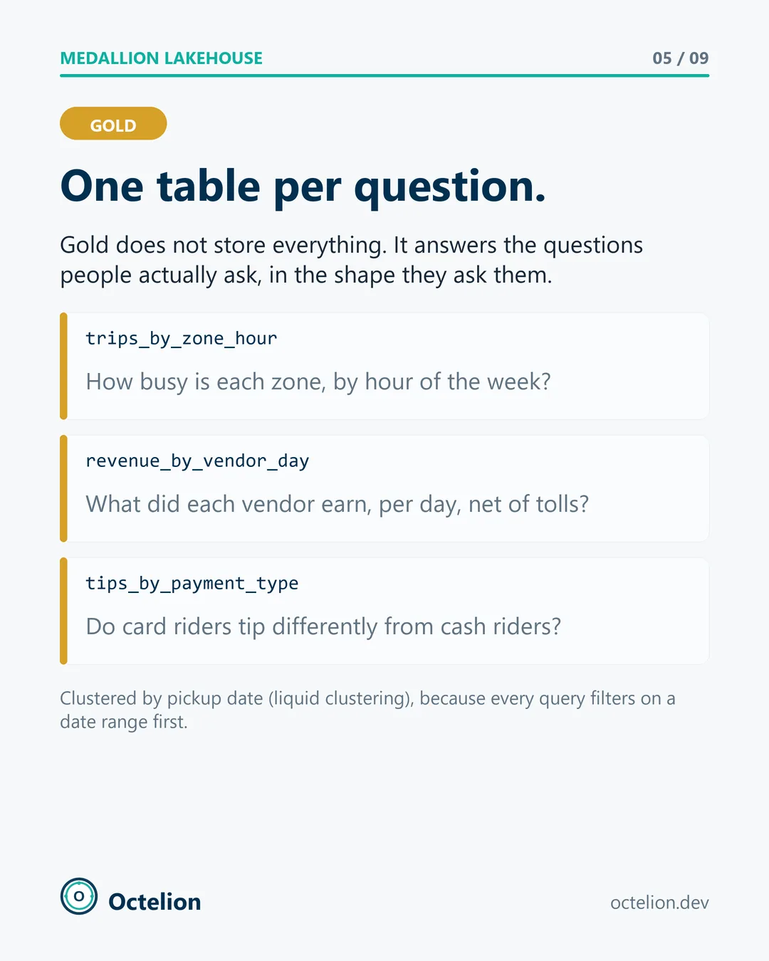
Gold does not store everything. It answers the questions people actually ask, in the shape they ask them: how busy each zone is by hour of the week, what each vendor code earned per day net of tolls, whether card riders tip differently from cash riders. The tables are clustered by pickup date, because every query filters on a date range first.
Two of the three need a note attached, and the June section below says why. The discipline is to resist a fourth table until someone asks the fourth question. Gold grows by request, not by anticipation.
Who can read what
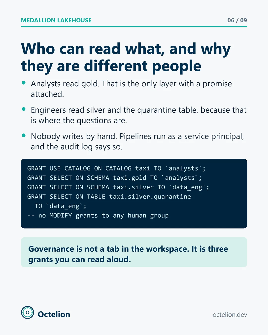
Analysts read gold, because gold is the only layer with a promise attached. Engineers read silver and the quarantine table, because that is where the questions are. Nobody writes by hand. The pipelines run as a service principal and the audit log says so. The whole policy is three Unity Catalog grants that can be read aloud, with no MODIFY grant to any human group. Governance is not a tab in the workspace.
GRANT USE CATALOG ON CATALOG taxi TO `analysts`;
GRANT SELECT ON SCHEMA taxi.gold TO `analysts`;
GRANT SELECT ON SCHEMA taxi.silver TO `data_eng`;
GRANT SELECT ON TABLE taxi.silver.quarantine TO `data_eng`;
-- no MODIFY grants to any human group
What the daily run costs
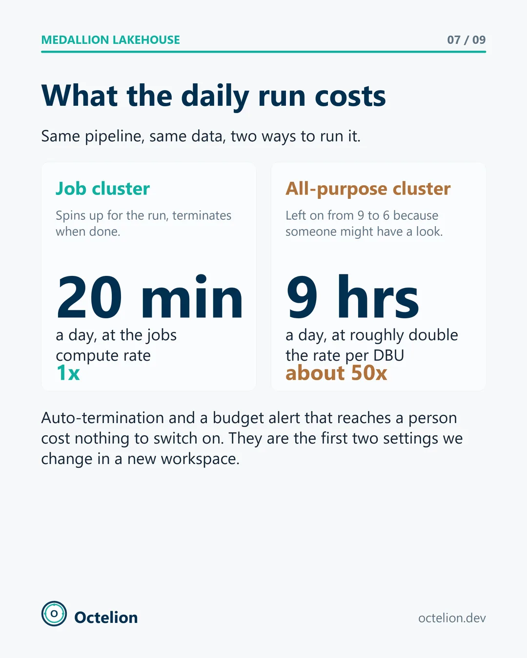
The same pipeline, on the same data, can be run two ways. A job cluster spins up for the run and terminates when it is done. An all-purpose cluster is left on from nine to six because someone might have a look. Jobs compute is billed at roughly half the all-purpose rate per DBU, so twenty minutes of the first against nine hours of the second (27 times the hours, about twice the rate) works out to roughly fifty times. The figures on the slide are that arithmetic on list rates, not a bill, and yours will differ. Auto-termination and a budget alert that reaches a person cost nothing to switch on, and they are the first two settings we change in a new workspace.
What breaks first, and how the pipeline tells you
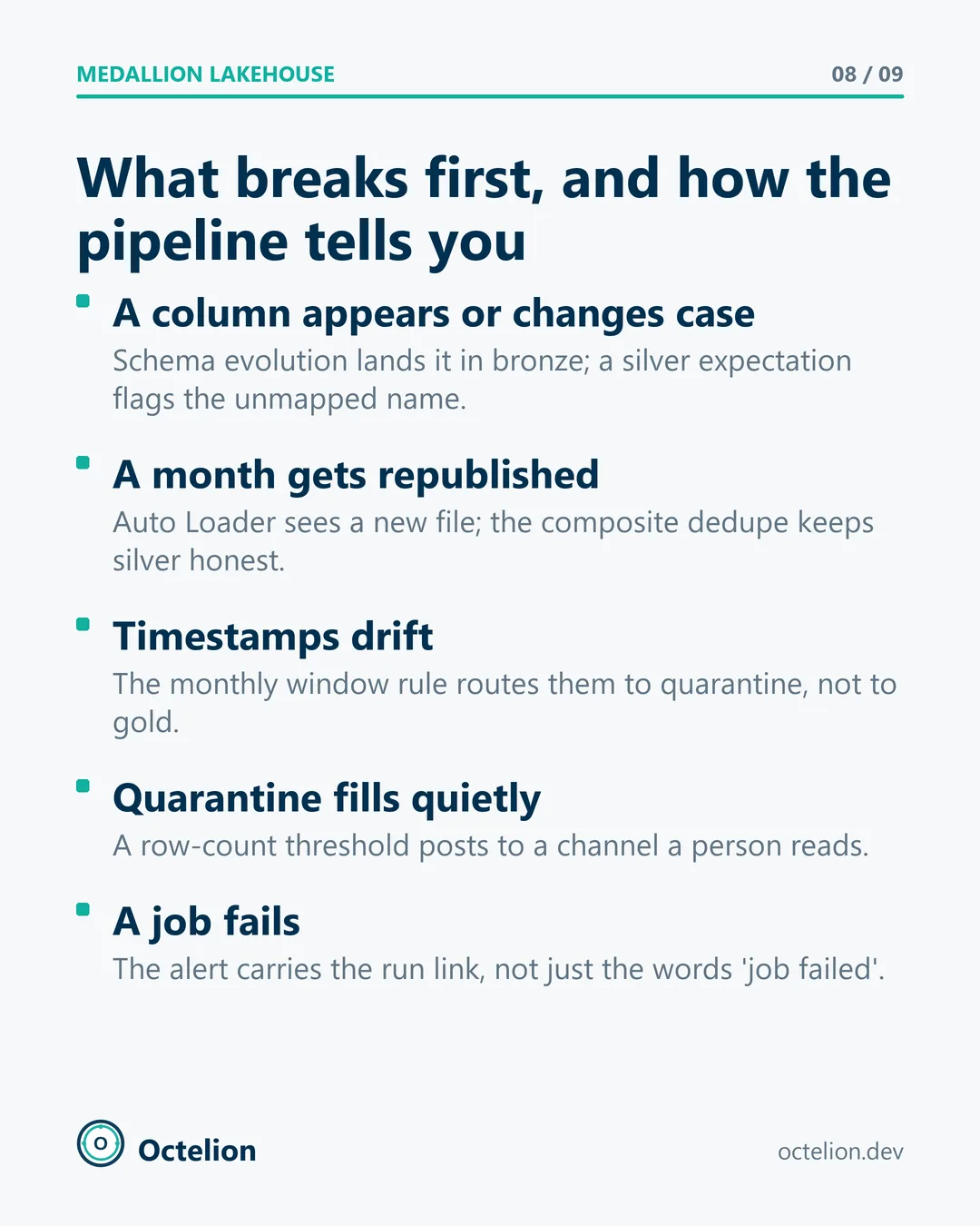
A column appears or changes case: schema evolution lands it in bronze and a silver expectation flags the unmapped name. A month gets republished under the same name: with allowOverwrites on, Auto Loader picks the file up again and the composite dedupe keeps silver honest. Timestamps drift: the monthly window rule routes them to quarantine, not to gold. Quarantine fills quietly: a row-count threshold posts to a channel a person reads. A job fails: the alert carries the run link, not just the words "job failed".
None of these is exotic. All of them happen in the first quarter of any real pipeline. The difference between a platform people trust and one they route around is whether the pipeline tells you, or a customer does.
What we found in June 2025
To check the rules against a real month, we read the June 2025 yellow taxi file straight over HTTP with DuckDB, no download, no cluster. The whole set of aggregates took about 27 seconds on a laptop. The query for pickups by hour is the shape every gold table starts from:
SELECT hour(tpep_pickup_datetime) AS h, count(*) AS trips
FROM read_parquet('https://d37ci6vzurychx.cloudfront.net/trip-data/yellow_tripdata_2025-06.parquet')
WHERE tpep_pickup_datetime >= '2025-06-01'
  AND tpep_pickup_datetime <  '2025-07-01'
  AND fare_amount >= 0
  AND tpep_dropoff_datetime >= tpep_pickup_datetime
GROUP BY 1 ORDER BY 1;
Swap the grouping column for the pickup location id and join the zone lookup to get the busiest zones. Swap it for payment type and average the tip column to get the tipping result, footnote included.
The file holds 4,322,960 rows. Twenty have a pickup outside June. 275,565 rows, 6.4% of the file, carry a negative fare; they are refunds and voids, and summing revenue without a rule for them is wrong by millions. 55,126 rows show zero distance and a fare over 20 dollars. 1,380 trips last more than three hours. 231 drop off before they pick up. 468 rows are duplicates on vendor, both timestamps, distance, fare and both zones. Each of those counts is a silver rule: duplicates are dropped, the rest land in the quarantine table. The clean set behind every chart on this page and on the home page keeps the rows with a pickup inside June, a fare of zero or more and a drop-off at or after the pickup: 4,047,145 rows, so 275,815 are dropped before any chart is drawn. A row can fail more than one rule, which is why that figure is smaller than the rule counts added together.
The chart of pickups by hour draws with JavaScript. The numbers are in the caption and in the data file linked below.
The clean rows say ordinary things clearly. The busiest pickup zone is JFK Airport with 175,520 pickups, ahead of Upper East Side South at 173,630 and Midtown Center at 170,390. Across the Midtown zones together, the 6 pm hour has 40,765 pickups and the 4 am hour has 1,803, about 22 times fewer. A trip of 2 to 3 miles takes 11 minutes at 4 am and 19 minutes between 11 am and 3 pm. A JFK pickup averages a 63.73 dollar fare and 45 minutes; LaGuardia, 45.08 dollars and 31 minutes.
One number argues for a rule we have not written yet. Average the recorded distance by pickup hour and the 5 am hour comes out at 41.6 miles, against 5 to 7 miles for most of the day, while its average fare is 26.25 dollars, only a few dollars above the rest. A handful of impossible distances is enough to move an hourly mean, and the fare column does not carry the error, so a chart of one without the other looks right and is not. That is a distance cap waiting to be added to silver, with its own quarantine count.
Two more numbers need a footnote, and both belong on the gold tables that carry them. Vendor code 2 appears on 78% of the clean rows. The column does not name a taxi company; it names the company that built the meter, so a table called revenue by vendor is about meter suppliers and should say so. Card riders tip 4.45 dollars on average, 28.6% of the fare, while cash riders tip zero in every row, because cash tips are not recorded by the meter. The data cannot say whether cash riders tip. That is a data problem, not a behaviour, and the gold table has to carry the footnote, or someone will present it as a finding.
The dataset changes. The discipline does not.

The same four layers run sales, support tickets or sensor data. Land everything with its provenance. Fix what can be fixed, quarantine the rest, and keep the count. Serve one table per question. Let three grants say who reads what. Switch on the alert that reaches a person. Swap the dataset and keep the rules.
The queries behind the home page
The five answers the home page gives come from these five queries. The June 2025 file is read straight over HTTP with read_parquet, no download, and the zone names come from the TLC's zone lookup CSV. All of it ran in about 27 seconds. Every query applies the same clean filter: a pickup inside June, a fare of zero or more and a drop-off at or after the pickup.
CREATE TABLE trips AS SELECT * FROM read_parquet(
  'https://d37ci6vzurychx.cloudfront.net/trip-data/yellow_tripdata_2025-06.parquet');
CREATE TABLE zones AS SELECT * FROM read_csv_auto(
  'https://d37ci6vzurychx.cloudfront.net/misc/taxi_zone_lookup.csv');
Midtown pickups by hour
SELECT hour(tpep_pickup_datetime) AS h, count(*) AS trips
FROM trips t JOIN zones z ON t.PULocationID = z.LocationID
WHERE tpep_pickup_datetime >= '2025-06-01'
  AND tpep_pickup_datetime <  '2025-07-01'
  AND fare_amount >= 0
  AND tpep_dropoff_datetime >= tpep_pickup_datetime
  AND z.Zone LIKE 'Midtown%'
GROUP BY 1 ORDER BY 1;
Tips by payment type
SELECT CASE payment_type WHEN 1 THEN 'card' WHEN 2 THEN 'cash' END AS p,
       avg(tip_amount) AS tip,
       avg(CASE WHEN fare_amount > 0 THEN tip_amount / fare_amount END) AS tip_share
FROM trips
WHERE tpep_pickup_datetime >= '2025-06-01'
  AND tpep_pickup_datetime <  '2025-07-01'
  AND fare_amount >= 0
  AND tpep_dropoff_datetime >= tpep_pickup_datetime
  AND payment_type IN (1, 2)
GROUP BY 1;
Minutes for a 2 to 3 mile trip, by hour
SELECT hour(tpep_pickup_datetime) AS h,
       avg(epoch(tpep_dropoff_datetime - tpep_pickup_datetime)) / 60 AS minutes
FROM trips
WHERE tpep_pickup_datetime >= '2025-06-01'
  AND tpep_pickup_datetime <  '2025-07-01'
  AND fare_amount >= 0
  AND tpep_dropoff_datetime >= tpep_pickup_datetime
  AND trip_distance BETWEEN 2 AND 3
GROUP BY 1 ORDER BY 1;
Top pickup zones
SELECT z.Zone, count(*) AS c
FROM trips t JOIN zones z ON t.PULocationID = z.LocationID
WHERE tpep_pickup_datetime >= '2025-06-01'
  AND tpep_pickup_datetime <  '2025-07-01'
  AND fare_amount >= 0
  AND tpep_dropoff_datetime >= tpep_pickup_datetime
GROUP BY 1 ORDER BY c DESC LIMIT 10;
Quality rules
The rules run on the whole file, not the clean set, because they are what decides which rows are clean.
SELECT count(*) FILTER (WHERE fare_amount < 0) AS negative_fare,
       count(*) FILTER (WHERE trip_distance = 0 AND fare_amount > 20) AS zero_distance_with_fare,
       count(*) FILTER (WHERE tpep_dropoff_datetime - tpep_pickup_datetime > INTERVAL 3 HOUR) AS over_three_hours,
       count(*) FILTER (WHERE tpep_dropoff_datetime < tpep_pickup_datetime) AS dropoff_before_pickup,
       count(*) - count(DISTINCT (VendorID, tpep_pickup_datetime, tpep_dropoff_datetime,
                                  trip_distance, fare_amount, PULocationID, DOLocationID)) AS duplicates
FROM trips;